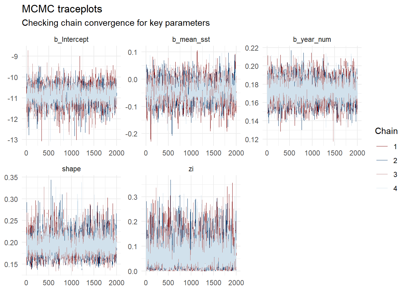
Figure S1. MCMC Traceplots for key model parameters.
The traceplots demonstrate the sampling behavior of the four independent Markov Chain Monte Carlo (MCMC) chains (represented by different colors) over 2000 post-warmup iterations. For all key parameters, including the fixed effects (b_Intercept, b_mean_sst, b_rok_num) and distributional parameters (shape, zi), the chains are stationary, well-mixed, and tightly overlapping. There are no visible divergent transitions or flatlining, which visually confirms excellent convergence of the sampling algorithm to the target posterior distribution.
Show the code
mcmc_rank_overlay(posterior, pars = parameters) +labs(title ="Rank histograms", subtitle ="Modern check for chain mixing") +theme_minimal()
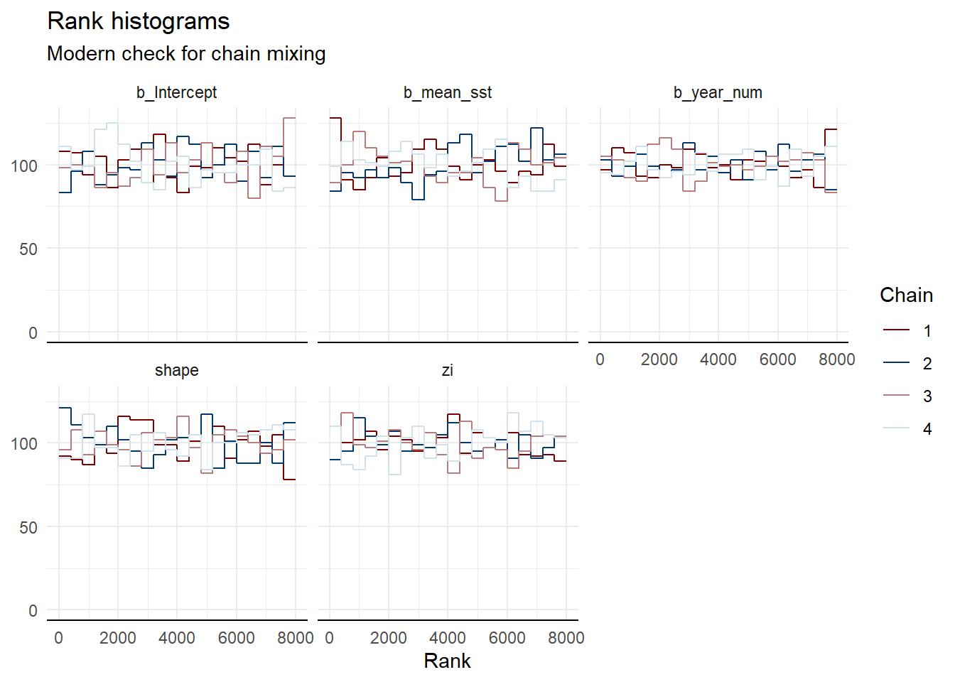
Figure S2. Rank overlay histograms for chain mixing.
Rank histograms provide a modern diagnostic for assessing MCMC chain convergence. The plot shows the distribution of ranked posterior draws across the four chains. For all evaluated parameters, the rank distributions are approximately uniform, and the chains overlap almost perfectly without any single chain dominating specific rank percentiles. This provides strong evidence that all chains have explored the same parameter space efficiently and achieved proper mixing.
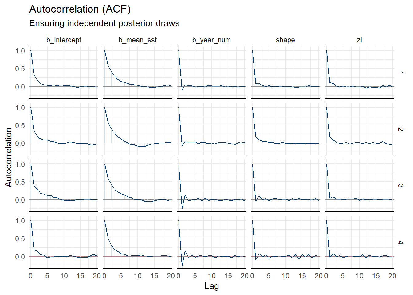
Figure S3. Autocorrelation Function (ACF) of posterior draws.
The ACF plots illustrate the correlation of the MCMC samples within each chain as a function of the lag distance. For all key parameters, the autocorrelation drops rapidly toward zero within the first few lags. This rapid decay indicates that the posterior draws are practically independent, leading to high effective sample size (ESS) values and confirming that the Hamiltonian Monte Carlo (HMC) sampler implemented in Stan operated with high efficiency.
Model evaluation (LOO-CV)
Before interpreting the epidemiological and physical effects, the predictive performance of the final zero-inflated negative ninomial (ZINB) model was evaluated using leave-one-out cross-validation (LOO-CV).
The evaluation confirmed the high numerical stability of the estimation. Analysis of the Pareto k diagnostic values revealed excellent robustness: 99.9% of the spatial observations yielded a value of k <= 0.7 (good status). The model exhibited a mean absolute error (MAE) of 0.081, indicating highly accurate baseline predictions. The negligible fraction of observations with high Pareto k values (0.07%) represents extreme, isolated spatiotemporal outliers (e.g., localized freak clusters of incidents) that do not skew the global posterior estimates.
Source Code
---title: "3. Diagnostics"engine: knitrformat: html: toc: true code-fold: true warning: false message: false---```{r}library(bayesplot)library(brms)library(ggplot2)library(dplyr)library(viridis)library(here)load(here::here("Data/data_for_the_model.RData"))fit_full_time_with_traffic <-readRDS(here::here("Fit/fit_full_time_with_traffic.rds"))color_scheme_set("mix-blue-red")posterior <-as.array(fit_full_time_with_traffic)parameters <-c("b_Intercept", "b_mean_sst", "b_year_num", "shape", "zi")mcmc_trace(posterior, pars = parameters) +labs(title ="MCMC traceplots", subtitle ="Checking chain convergence for key parameters") +theme_minimal()```Figure S1. MCMC Traceplots for key model parameters. The traceplots demonstrate the sampling behavior of the four independent Markov Chain Monte Carlo (MCMC) chains (represented by different colors) over 2000 post-warmup iterations. For all key parameters, including the fixed effects (b_Intercept, b_mean_sst, b_rok_num) and distributional parameters (shape, zi), the chains are stationary, well-mixed, and tightly overlapping. There are no visible divergent transitions or flatlining, which visually confirms excellent convergence of the sampling algorithm to the target posterior distribution.```{r}mcmc_rank_overlay(posterior, pars = parameters) +labs(title ="Rank histograms", subtitle ="Modern check for chain mixing") +theme_minimal()```Figure S2. Rank overlay histograms for chain mixing.Rank histograms provide a modern diagnostic for assessing MCMC chain convergence. The plot shows the distribution of ranked posterior draws across the four chains. For all evaluated parameters, the rank distributions are approximately uniform, and the chains overlap almost perfectly without any single chain dominating specific rank percentiles. This provides strong evidence that all chains have explored the same parameter space efficiently and achieved proper mixing.```{r}mcmc_acf(posterior, pars = parameters) +labs(title ="Autocorrelation (ACF)", subtitle ="Ensuring independent posterior draws") +theme_minimal()```Figure S3. Autocorrelation Function (ACF) of posterior draws. The ACF plots illustrate the correlation of the MCMC samples within each chain as a function of the lag distance. For all key parameters, the autocorrelation drops rapidly toward zero within the first few lags. This rapid decay indicates that the posterior draws are practically independent, leading to high effective sample size (ESS) values and confirming that the Hamiltonian Monte Carlo (HMC) sampler implemented in Stan operated with high efficiency.Model evaluation (LOO-CV)Before interpreting the epidemiological and physical effects, the predictive performance of the final zero-inflated negative ninomial (ZINB) model was evaluated using leave-one-out cross-validation (LOO-CV).```{r}library(brms)fit_full_time_with_traffic <-readRDS(here::here("Fit/fit_full_time_with_traffic.rds"))fit_full_time_with_traffic <-add_criterion(fit_full_time_with_traffic, "loo")loo_result <-loo(fit_full_time_with_traffic)print(loo_result)predictions <-fitted(fit_full_time_with_traffic, summary =TRUE)mae <-mean(abs(data$total_count - predictions[, "Estimate"]), na.rm =TRUE)cat("Mean absolute error (MAE):", round(mae, 3), "\n")```The evaluation confirmed the high numerical stability of the estimation. Analysis of the Pareto k diagnostic values revealed excellent robustness: 99.9% of the spatial observations yielded a value of k <= 0.7 (good status). The model exhibited a mean absolute error (MAE) of 0.081, indicating highly accurate baseline predictions. The negligible fraction of observations with high Pareto k values (0.07%) represents extreme, isolated spatiotemporal outliers (e.g., localized freak clusters of incidents) that do not skew the global posterior estimates.