1. Data Preparation and Exploratory Analysis

Overview of the dataset

The dataset integrates three primary data sources over the Baltic Sea region:

1. Accident records: Extracted from the EMSA EMCiP database (aggregated by month, year, and grid cell).

2. Exposure data (Traffic): Vessel traffic density derived from the Automatic Identification System (AIS).

3. Environmental data: Mean sea surface temperature (SST).

The spatial resolution is based on a defined grid system (longitude and latitude intervals), and the temporal resolution is monthly.

library(dplyr)
library(ggplot2)

# load data
load(here::here("Data/data_for_the_model.RData"))


glimpse(data %>% select(total_count, mean_sst, mean_traffic, month_factor, year_num))

Rows: 18,756
Columns: 5
$ total_count  <dbl> 0, 0, 0, 0, 0, 0, 0, 0, 0, 0, 0, 0, 0, 0, 0, 0, 0, 0, 0, …
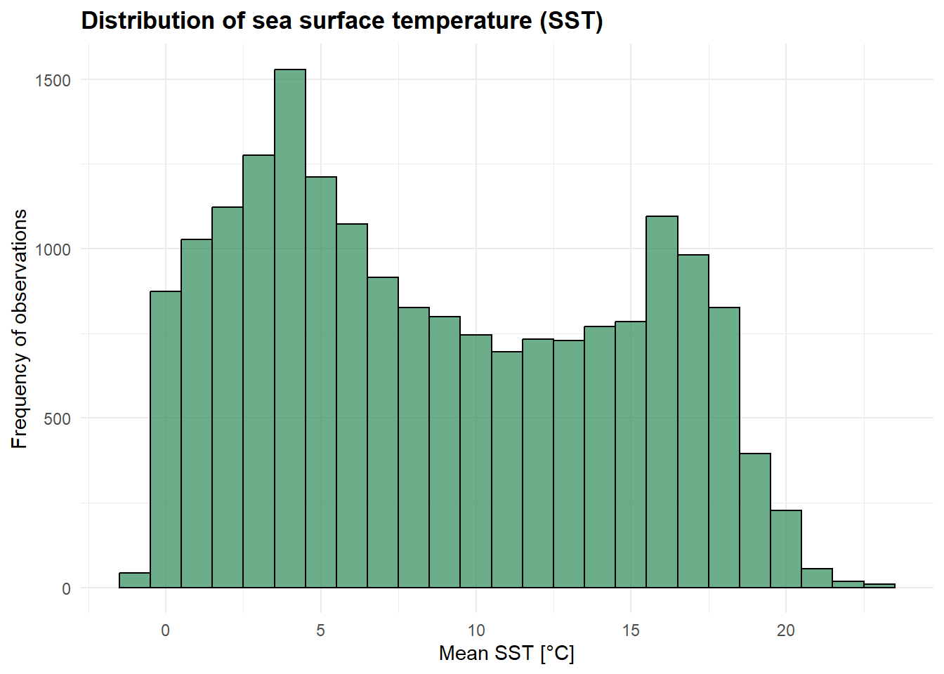
$ mean_sst     <dbl> 1.126774, 2.171232, 2.261398, 2.757355, 2.336804, 2.71901…
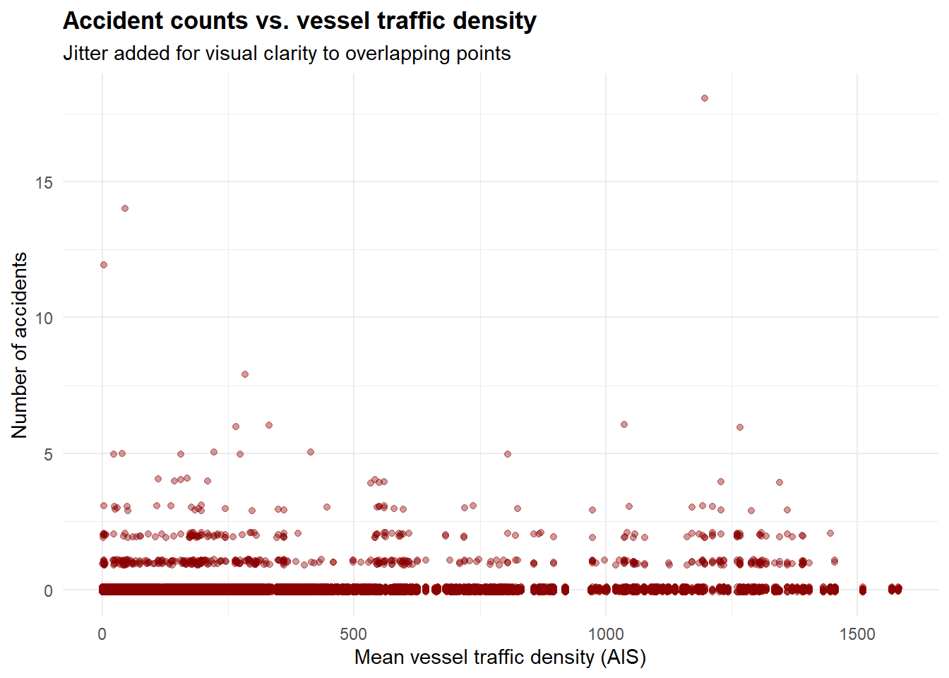
$ mean_traffic <dbl> 313.416087, 291.692347, 1339.565172, 666.018946, 1274.568…
$ month_factor <fct> Jan, Jan, Jan, Jan, Jan, Jan, Jan, Jan, Jan, Jan, Jan, Ja…
$ year_num     <dbl> 1, 1, 1, 1, 1, 1, 1, 1, 1, 1, 1, 1, 1, 1, 1, 1, 1, 1, 1, …

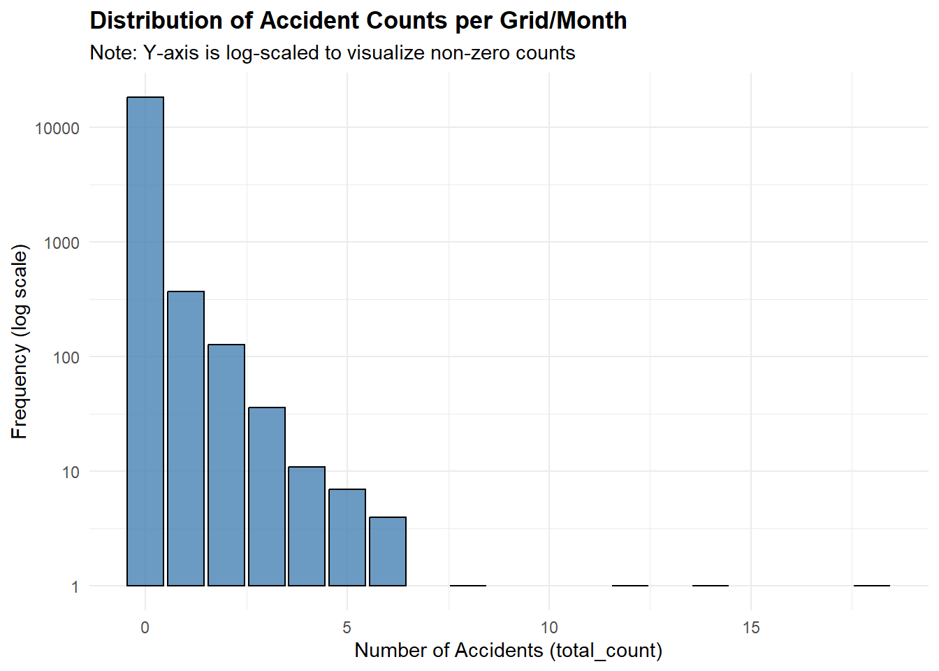
summary(data %>% select(total_count, mean_sst, mean_traffic))

  total_count          mean_sst       mean_traffic      
 Min.   : 0.00000   Min.   :-1.232   Min.   :   0.0044  
 1st Qu.: 0.00000   1st Qu.: 3.718   1st Qu.:  54.0508  
 Median : 0.00000   Median : 7.870   Median : 186.9045  
 Mean   : 0.04745   Mean   : 8.781   Mean   : 287.3643  
 3rd Qu.: 0.00000   3rd Qu.:14.124   3rd Qu.: 384.6163  
 Max.   :18.00000   Max.   :23.319   Max.   :1581.9298  

The “zero-inflation” problem The fundamental challenge in modeling maritime accidents is their rarity. Traditional Poisson or negative binomial models often fail because they cannot account for the massive excess of zeros (grid cells with no accidents in a given month).

The bar plot below illustrates the distribution of my response variable (total_count). The overwhelming dominance of zeros strictly justifies the deployment of a zero-inflated negative binomial (ZINB) modeling framework.

ggplot(data, aes(x = total_count)) +
  geom_bar(fill = "steelblue", color = "black", alpha = 0.8) +
  scale_y_log10() + 
  labs(
    title = "Distribution of Accident Counts per Grid/Month",
    subtitle = "Note: Y-axis is log-scaled to visualize non-zero counts",
    x = "Number of Accidents (total_count)",
    y = "Frequency (log scale)"
  ) +
  theme_minimal() +
  theme(plot.title = element_text(face = "bold"))

Exposure Variable: Vessel Traffic Density In spatial risk analysis, areas with higher traffic inherently carry a higher baseline risk of incidents. I use AIS-derived traffic density (mean_traffic) as an exposure offset in my Bayesian model.

The scatter plot below shows the relationship between traffic density and accident occurrence. As expected, accidents (values > 0) tend to cluster in grid cells with higher traffic volumes (such as the Danish Straits).

ggplot(data, aes(x = mean_traffic, y = total_count)) +
  geom_jitter(alpha = 0.4, color = "darkred", width = 0.1, height = 0.1) +
  labs(
    title = "Accident counts vs. vessel traffic density",
    subtitle = "Jitter added for visual clarity to overlapping points",
    x = "Mean vessel traffic density (AIS)",
    y = "Number of accidents"
  ) +
  theme_minimal() +
  theme(plot.title = element_text(face = "bold"))

Environmental variable: sea surface temperature (SST) Temperature is analyzed as a proxy for harsh winter conditions (e.g., icing, freezing spray). The distribution of SST across all spatiotemporal observations reflects the distinct seasonality of the Baltic Sea.

ggplot(data, aes(x = mean_sst)) +
  geom_histogram(binwidth = 1, fill = "seagreen", color = "black", alpha = 0.7) +
  labs(
    title = "Distribution of sea surface temperature (SST)",
    x = "Mean SST [°C]",
    y = "Frequency of observations"
  ) +
  theme_minimal() +
  theme(plot.title = element_text(face = "bold"))